Verteilung (mathematische Analyse)

Distributionen (oder verallgemeinerte Funktionen ) sind Objekte, die den klassischen Funktionsbegriff in der Analysis verallgemeinern . Sie ermöglichen die Differenzierung von Funktionen, deren Ableitungen im klassischen Sinne nicht existieren. Insbesondere besitzt jede lokal integrierbare Funktion eine distributionelle Ableitung. Distributionen finden breite Anwendung in der Theorie partieller Differentialgleichungen , wo die Existenz distributioneller Lösungen leichter zu beweisen ist als die klassischer Lösungen oder wo geeignete klassische Lösungen nicht existieren. Auch in Physik und Ingenieurwesen sind Distributionen von Bedeutung , da viele Probleme naturgemäß zu Differentialgleichungen führen, deren Lösungen oder Anfangsbedingungen Distributionen sind, wie beispielsweise die Dirac-Delta -Funktion.

Die praktische Anwendung von Distributionen lässt sich bis zur Verwendung von Greenschen Funktionen in den 1830er Jahren zur Lösung gewöhnlicher Differentialgleichungen zurückverfolgen , wurde aber erst viel später formalisiert. Laut Kolmogorov & Fomin (1957) gehen verallgemeinerte Funktionen auf die Arbeiten von Sergei Sobolev  ( 1936 ) zu hyperbolischen partiellen Differentialgleichungen zweiter Ordnung zurück, und Laurent Schwartz entwickelte die Ideen in den späten 1940er Jahren in erweiterter Form weiter. Seiner Autobiografie zufolge führte Schwartz den Begriff „Distribution“ in Analogie zur Verteilung elektrischer Ladung ein, wobei er möglicherweise nicht nur Punktladungen, sondern auch Dipole usw. einschloss. Gårding (1997) merkt an, dass die Ideen in Schwartz’ bahnbrechendem Buch (1951) zwar nicht völlig neu waren, aber Schwartz’ umfassender Ansatz und seine Überzeugung, dass Distributionen in der Analysis nahezu überall nützlich sein würden, den entscheidenden Unterschied ausmachten.

Die Distributionstheorie interpretiert Funktionen als lineare Funktionale, die auf einem Raum wirken.Testfunktionen . Standardfunktionen wirken durch Integration gegen eine Testfunktion, viele andere lineare Funktionale entstehen jedoch nicht auf diese Weise; diese werden als „verallgemeinerte Funktionen“ bezeichnet. Es gibt verschiedene Möglichkeiten, den Raum der Testfunktionen zu wählen, was zu unterschiedlichen Räumen von Distributionen führt. Der grundlegende Raum der Testfunktionen besteht aus glatten Funktionen mitkompaktem Träger, was zu Standarddistributionen führt. Die Verwendung des Raums glatter, schnell (schneller als jedes Polynom ansteigender) fallender Testfunktionen (diese Funktionen werdenSchwartz-Funktionen) liefert hingegen die temperierten Distributionen. Diese sind wichtig, da sie eine wohldefinierte distributionelle Fouriertransformation besitzen. Jede temperierte Distribution ist eine Distribution im üblichen Sinne, aber die Umkehrung gilt nicht: Im Allgemeinen gilt: Je größer der Raum der Testfunktionen, desto restriktiver ist der Begriff der Distribution. Andererseits führt die Verwendung von Räumen analytischer Testfunktionen zu Satos Theorie derHyperfunktionen; diese Theorie unterscheidet sich von den vorherigen, da es keine analytischen Funktionen mit nichtleerem kompaktem Träger gibt.

Distributionen sind eine Klasse linearer Funktionale , die eine Menge von Testfunktionen (konventionelle und wohldefinierte Funktionen) auf die Menge der reellen Zahlen abbilden. Im einfachsten Fall ist die betrachtete Menge der Testfunktionen D( ℝ ), d. h. die Menge der Funktionen  : ℝ → ℝ mit zwei Eigenschaften: ${\displaystyle \varphi }$

• ${\displaystyle \varphi }$ist glatt (unendlich oft differenzierbar);
• ${\displaystyle \varphi }$besitzt kompakten Träger (ist außerhalb eines begrenzten Intervalls identisch null).

Eine Verteilung T ist eine lineare Abbildung T  : D( R ) → R. Anstatt T ( ) zu schreiben, ist es üblich, für den Wert von T, der auf eine Testfunktion angewendet wird, T (x) zu schreiben . Ein einfaches Beispiel für eine Verteilung ist die Dirac-Delta-Verteilung δ , definiert durch ${\displaystyle \varphi }$${\displaystyle \langle T,\varphi \rangle }$${\displaystyle \varphi }$

${\displaystyle \left\langle \delta ,\varphi \right\rangle =\varphi (0),}$

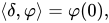
Das bedeutet, dass δ eine Testfunktion bei 0 auswertet. Physikalisch lässt sich dies als die Dichte einer Punktquelle interpretieren.

Wie im Folgenden beschrieben, gibt es einfache Abbildungen sowohl von lokal integrierbaren Funktionen als auch von Radon-Maßen auf entsprechende Verteilungen, aber nicht alle Verteilungen können auf diese Weise gebildet werden.

Sei f  : R → R eine lokal integrierbare Funktion . Dann kann eine entsprechende Distribution T _f definiert werden durch

${\displaystyle \left\langle T_{f},\varphi \right\rangle =\int _{\mathbf {R} }f(x)\varphi (x)\,dx\quad {\text{for}}\quad \varphi \in D(\mathbf {R} ).}$

Dieses Integral ist eine reelle Zahl , die linear und stetig von abhängt . Umgekehrt bestimmen die Werte der Verteilung T_{_f} auf Testfunktionen in D( ℝ ) die punktweise fast überall gültigen Werte der Funktion f auf ℝ . In einer gängigen , wenn auch nicht immer eindeutigen Notation wird f oft sowohl für die ursprüngliche Funktion f als auch für die zugehörige Verteilung T _{_f} verwendet . Dieses Beispiel legt die Definition einer Verteilung als lineares und, in einem geeigneten Sinne, stetiges Funktional auf dem Raum der Testfunktionen D( ℝ ) nahe. ${\displaystyle \varphi }$

Analog dazu kann, wenn μ ein Radon-Maß auf R ist , eine entsprechende Verteilung R _μ definiert werden durch

${\displaystyle \left\langle R_{\mu },\varphi \right\rangle =\int _{\mathbf {R} }\varphi \,d\mu \quad {\text{for}}\quad \varphi \in D(\mathbf {R} ).}$

Dieses Integral hängt auch linear und stetig von ab , sodass R _μ eine Distribution ist. Wenn μ absolut stetig bezüglich des Lebesgue-Maßes mit Dichte f und d μ = f dx ist , dann ist diese Definition für R _μ dieselbe wie die vorherige für T _f . Wenn μ jedoch nicht absolut stetig ist, dann ist R _μ eine Distribution, die keiner Funktion zugeordnet ist. Wenn beispielsweise P das Punktmassenmaß auf R ist , das der einelementigen Menge {0} das Maß eins und Mengen, die nicht Null enthalten, das Maß null zuordnet, dann ${\displaystyle \varphi }$

${\displaystyle \int _{\mathbf {R} }\varphi \,dP=\varphi (0),}$

so dass R _P = δ das Dirac-Delta ist.

Distributionen lassen sich mit reellen Zahlen multiplizieren und addieren, sodass sie einen reellen Vektorraum bilden . Sie lassen sich auch mit unendlich oft differenzierbaren Funktionen multiplizieren. Es ist jedoch nicht möglich, ein Produkt allgemeiner Distributionen zu definieren , das die übliche punktweise Produktbildung von Funktionen erweitert und dieselben algebraischen Eigenschaften aufweist. Dieses Ergebnis wurde von Schwartz (1954) bewiesen und wird üblicherweise als Satz von Schwartz bezeichnet .

Es ist wünschenswert, eine Definition für die Ableitung einer Distribution zu wählen, die – zumindest für Distributionen, die von glatten Funktionen abgeleitet sind – die Eigenschaft besitzt, dass . Wenn eine Testfunktion ist, können wir durch partielle Integration zeigen, dass ${\displaystyle T'_{f}=T_{f'}}$${\displaystyle \varphi }$

${\displaystyle \left\langle f',\varphi \right\rangle =\int _{\mathbf {R} }f'\varphi \,dx={\Big [}f(x)\varphi (x){\Big ]}_{-\infty }^{\infty }-\int _{\mathbf {R} }f\varphi '\,dx=-\left\langle f,\varphi '\right\rangle }$

Die letzte Gleichheit folgt daraus, dass kompakten Träger besitzt und somit außerhalb einer beschränkten Menge null ist. Dies legt nahe, dass wir, falls eine Distribution ist, ihre Ableitung wie folgt definieren sollten :${\displaystyle \varphi }$${\displaystyle T}$${\displaystyle T'}$

${\displaystyle \left\langle T',\varphi \right\rangle =-\left\langle T,\varphi '\right\rangle .}$

Es stellt sich heraus, dass dies die korrekte Definition ist; sie erweitert die gewöhnliche Definition der Ableitung, jede Distribution wird unendlich oft differenzierbar und die üblichen Eigenschaften von Ableitungen bleiben erhalten.

Beispiel: Erinnern Sie sich daran, dass die Dirac-Delta-Funktion (auch Dirac-Delta-Funktion genannt) die durch die Gleichung definierte Verteilung ist.

${\displaystyle \left\langle \delta ,\varphi \right\rangle =\varphi (0).}$

Es handelt sich um die Ableitung der Verteilung, die der Heaviside-Sprungfunktion H entspricht : Für jede Testfunktion , ${\displaystyle \varphi }$

${\displaystyle \left\langle H',\varphi \right\rangle =-\int _{-\infty }^{\infty }H(x)\varphi '(x)\,dx=-\varphi (\infty )+\varphi (0)=\left\langle \delta ,\varphi \right\rangle ,}$

Also ist H ′ = δ . Beachte, dass (∞) = 0 gilt, da H′ gemäß unserer Definition einer Testfunktion kompakten Träger besitzt. Analog dazu ist die Ableitung des Dirac-Deltas die durch die Gleichung definierte Distribution. ${\displaystyle \varphi }$${\displaystyle \varphi }$

${\displaystyle \langle \delta ',\varphi \rangle =-\varphi '(0).}$

Diese letztgenannte Verteilung ist ein Beispiel für eine Verteilung, die nicht von einer Funktion oder einem Maß abgeleitet ist. Ihre physikalische Interpretation ist die Dichte einer Dipolquelle. So wie der Dirac-Impuls im schwachen Grenzfall als Folge verschiedener Arten von Auslenkungsfunktionen mit konstanter Norm, stetig zunehmender Amplitude und abnehmendem Träger realisiert werden kann, lässt sich seine Ableitung definitionsgemäß als schwacher Grenzwert der negativen Ableitungen dieser Funktionen realisieren, die nun antisymmetrisch um den singulären Trägerpunkt der resultierenden Verteilung sind.

Im Folgenden werden reellwertige Distributionen auf einer offenen Teilmenge U von ℝⁿ formal definiert. Mit ^{geringfügigen} Modifikationen lassen sich auch komplexwertige Distributionen definieren, und ℝⁿ kann durch ^eine beliebige ( parakompakte ) glatte Mannigfaltigkeit ersetzt werden .

Zunächst muss der Raum D( U ) der Testfunktionen auf U definiert werden . Anschließend muss ihm eine Topologie zugewiesen werden, indem der Grenzwert einer Folge von Elementen aus D( U ) definiert wird. Der Raum der Distributionen ergibt sich dann als der Raum der stetigen linearen Funktionale auf D( U ).

The space D(U) of test functions on U is defined as follows. A function ${\displaystyle \varphi }$ : U → R is said to have compact support if there exists a compact subset K of U such that ${\displaystyle \varphi }$(x) = 0 for all x in U \ K. The elements of D(U) are the infinitely differentiable functions ${\displaystyle \varphi }$ : U → R with compact support – also known as bump functions. This is a real vector space. It can be given a topology by defining the limit of a sequence of elements of D(U). A sequence (${\displaystyle \varphi }$_k) in D(U) is said to converge to ${\displaystyle \varphi }$ ∈ D(U) if the following two conditions hold:^[1]

• There is a compact set K ⊂ U containing the supports of all ${\displaystyle \varphi }$_k:

${\displaystyle \bigcup \nolimits _{k}\operatorname {supp} (\varphi _{k})\subset K.}$

• For each multi-index α, the sequence of partial derivatives ${\displaystyle \partial ^{\alpha }\varphi _{k}}$ tends uniformly to ${\displaystyle \partial ^{\alpha }\varphi }$.

With this definition, D(U) becomes a completelocally convextopological vector space satisfying the Heine–Borel property.^[2]

This topology can be placed in the context of the following general construction: let

${\displaystyle X=\bigcup \nolimits _{i}X_{i}}$

be a countable increasing union of locally convex topological vector spaces and ι_i : X_i → X be the inclusion maps. In this context, the inductive limit topology, or final topology, τ on X is the finest locally convex vector space topology making all the inclusion maps ${\displaystyle \iota _{i}}$ continuous. The topology τ can be explicitly described as follows: let β be the collection of convex balanced subsets W of X such that W ∩ X_i is open for all i. A base for the inductive limit topology τ then consists of the sets of the form x + W, where x in X and W in β.

The proof that τ is a vector space topology makes use of the assumption that each X_i is locally convex. By construction, β is a local base for τ. That any locally convex vector space topology on X must necessarily contain τ means it is the weakest one. One can also show that, for each i, the subspace topology X_i inherits from τ coincides with its original topology. When each X_i is a Fréchet space, (X, τ) is called an LF space.

Now let U be the union of U_i where {U_i} is a countable nested family of open subsets of U with compact closures K_i = U_i. Then we have the countable increasing union

${\displaystyle \mathrm {D} (U)=\bigcup \nolimits _{i}\mathrm {D} _{K_{i}}}$

where D_Ki is the set of all smooth functions on U with support lying in K_i. On each D_Ki, consider the topology given by the seminorms

${\displaystyle \|\varphi \|_{\alpha }=\max _{x\in K_{i}}\left|\partial ^{\alpha }\varphi \right|,}$

i.e. the topology of uniform convergence of derivatives of arbitrary order. This makes each D_Ki a Fréchet space. The resulting LF space structure on D(U) is the topology described in the beginning of the section.

On D(U), one can also consider the topology given by the seminorms

${\displaystyle \|\varphi \|_{\alpha ,K_{i}}=\max _{x\in K_{i}}\left|\partial ^{\alpha }\varphi \right|.}$

However, this topology has the disadvantage of not being complete. On the other hand, because of the particular features of D_Ki's, a set this bounded with respect to τ if and only if it lies in some D_Ki's. The completeness of (D(U), τ) then follow from that of D_Ki's.

The topology τ is not metrizable by the Baire category theorem, since D(U) is the union of subspaces of the first category in D(U).^[3]

A distribution on U is a continuous linear functionalT : D(U) → R (or T : D(U) → C). That is, a distribution T assigns to each test function ${\displaystyle \varphi }$ a real (or complex) scalar T(${\displaystyle \varphi }$) such that

${\displaystyle T(c_{1}\varphi _{1}+c_{2}\varphi _{2})=c_{1}T(\varphi _{1})+c_{2}T(\varphi _{2})}$

for all test functions ${\displaystyle \varphi }$₁, ${\displaystyle \varphi }$₂ and scalars c₁, c₂. Moreover, T is continuous if and only if

${\displaystyle \lim _{k\to \infty }T(\varphi _{k})=T{\Bigl (}\lim _{k\to \infty }\varphi _{k}{\Bigr )}}$

for every convergent sequence ${\displaystyle \varphi }$_k in D(U). (Even though the topology of D(U) is not metrizable, a linear functional on D(U) is continuous if and only if it is sequentially continuous.) Equivalently, T is continuous if and only if for every compact subset K of U there exists a positive constant C_K and a non-negative integer N_K such that

${\displaystyle |T(\varphi )|\leq C_{K}\sup {\bigl \{}|\partial ^{\alpha }\varphi (x)|\mathrel {\big |} x\in K,|\alpha |\leq N_{K}{\bigr \}}}$

for all test functions ${\displaystyle \varphi }$ with support contained in K.^[4]

The space of distributions on U is denoted by D′(U) and it is the continuous dual space of D(U). No matter what dual topology is placed on D′(U), a sequence of distributions converges in this topology if and only if it converges pointwise (although this need not be true of a net), which is why the topology is sometimes defined to be the weak-* topology. But often the topology of bounded convergence, which in this case is the same as the topology of uniform convergence on compact sets, is placed on D′(U) since it is with this topology that D′(U) becomes a nuclearMontel space and it is with this topology that the kernels theorem of Schwartz holds.^[5] No matter which topology is chosen, D′(U) will be a non-metrizable, locally convex topological vector space.

The duality pairing between a distribution T in D′(U) and a test function ${\displaystyle \varphi }$ in D(U) is denoted using angle brackets by

${\displaystyle {\begin{cases}\mathrm {D} '(U)\times \mathrm {D} (U)\to \mathbf {R} \\(T,\varphi )\mapsto \langle T,\varphi \rangle ,\end{cases}}}$

so that ⟨T,${\displaystyle \varphi }$⟩ = T(${\displaystyle \varphi }$). One interprets this notation as the distribution T acting on the test function ${\displaystyle \varphi }$ to give a scalar, or symmetrically as the test function ${\displaystyle \varphi }$ acting on the distribution T.

A sequence of distributions (T_k) converges with respect to the weak-* topology on D′(U) to a distribution T if and only if

${\displaystyle \langle T_{k},\varphi \rangle \to \langle T,\varphi \rangle }$

for every test function ${\displaystyle \varphi }$ in D(U). For example, if f_k : R → R is the function

${\displaystyle f_{k}(x)={\begin{cases}k&{\text{if}}\ 0\leq x\leq 1/k\\0&{\text{otherwise}}\end{cases}}}$

and T_k is the distribution corresponding to f_k, then

${\displaystyle \langle T_{k},\varphi \rangle =k\int _{0}^{1/k}\varphi (x)\,dx\to \varphi (0)=\langle \delta ,\varphi \rangle }$

as k → ∞, so T_k → δ in D′(R). Thus, for large k, the function f_k can be regarded as an approximation of the Dirac delta distribution.

The function f : U → R is called locally integrable if it is Lebesgue integrable over every compact subset K of U.^[6] This is a large class of functions which includes all continuous functions and all L^p functions. The topology on D(U) is defined in such a fashion that any locally integrable function f yields a continuous linear functional on D(U) – that is, an element of D′(U) – denoted here by T_f, whose value on the test function ${\displaystyle \varphi }$ is given by the Lebesgue integral:

${\displaystyle \langle T_{f},\varphi \rangle =\int _{U}f\varphi \,dx.}$

Conventionally, one abuses notation by identifying T_f with f, provided no confusion can arise, and thus the pairing between T_f and ${\displaystyle \varphi }$ is often written

${\displaystyle \langle f,\varphi \rangle =\langle T_{f},\varphi \rangle .}$

If f and g are two locally integrable functions, then the associated distributions T_f and T_g are equal to the same element of D′(U) if and only if f and g are equal almost everywhere (see, for instance, Hörmander (1983, Theorem 1.2.5)). In a similar manner, every Radon measure μ on U defines an element of D′(U) whose value on the test function ${\displaystyle \varphi }$ is ∫${\displaystyle \varphi }$ dμ. As above, it is conventional to abuse notation and write the pairing between a Radon measure μ and a test function ${\displaystyle \varphi }$ as ${\displaystyle \langle \mu ,\varphi \rangle }$. Conversely, as shown in a theorem by Schwartz (similar to the Riesz representation theorem), every distribution which is non-negative on non-negative functions is of this form for some (positive) Radon measure.

The test functions are themselves locally integrable, and so define distributions. As such they are dense in D′(U) with respect to the topology on D′(U) in the sense that for any distribution T ∈ D′(U), there is a net ${\displaystyle \varphi }$_i ∈ D(U) such that

${\displaystyle \langle \varphi _{i},\psi \rangle \to \langle T,\psi \rangle }$

for all Ψ ∈ D(U). This fact follows from the Hahn–Banach theorem, since the dual of D′(U) with its weak-* topology is the space D(U).^[7] A stronger result of sequential density can be proven more constructively by a convolution argument.

Many operations which are defined on smooth functions with compact support can also be defined for distributions. In general, if A : D(U) → D(U) is a linear mapping of vector spaces which is continuous with respect to the weak-* topology, then it is possible to extend A to a mapping A : D′(U) → D′(U) by passing to the limit. (This approach works for non-linear mappings as well, provided they are assumed to be uniformly continuous.)

In practice, however, it is more convenient to define operations on distributions by means of the transpose.^[8] If A : D(U) → D(U) is a continuous linear operator, then the transpose is an operator A^t : D(U) → D(U) such that

${\displaystyle \int _{U}A\varphi (x)\cdot \psi (x)\,dx=\int _{U}\varphi (x)\cdot A^{t}\psi (x)\,dx\qquad {\text{for all}}\ \varphi ,\psi \in D(U).}$

(For operators acting on spaces of complex-valued test functions, the transpose A^t differs from the adjoint A^* in that it does not include a complex conjugate.)

If such an operator A^t exists and is continuous on D(U), then the original operator A may be extended to D′(U) by defining AT for a distribution T as

${\displaystyle \langle AT,\varphi \rangle =\langle T,A^{t}\varphi \rangle \qquad {\text{for all}}\ \varphi \in D(U).}$

Suppose A : D(U) → D(U) is the partial derivative operator

${\displaystyle A\varphi ={\frac {\partial \varphi }{\partial x_{k}}}.}$

If ${\displaystyle \varphi }$ and ψ are in D(U), then an integration by parts gives

${\displaystyle \int _{U}{\frac {\partial \varphi }{\partial x_{k}}}\psi \,dx=-\int _{U}\varphi {\frac {\partial \psi }{\partial x_{k}}}\,dx,}$

so that A^t = −A. This operator is a continuous linear transformation on D(U). So, if T ∈ D′(U) is a distribution, then the partial derivative of T with respect to the coordinate x_k is defined by the formula

${\displaystyle \left\langle {\frac {\partial T}{\partial x_{k}}},\varphi \right\rangle =-\left\langle T,{\frac {\partial \varphi }{\partial x_{k}}}\right\rangle \qquad {\text{for all}}\ \varphi \in D(U).}$

With this definition, every distribution is infinitely differentiable, and the derivative in the direction x_k is a linear operator on D′(U).

More generally, if α = (α₁, ..., α_n) is an arbitrary multi-index and ∂^α is the associated partial derivative operator, then the partial derivative ∂^αT of the distribution T ∈ D′(U) is defined by

${\displaystyle \left\langle \partial ^{\alpha }T,\varphi \right\rangle =(-1)^{|\alpha |}\left\langle T,\partial ^{\alpha }\varphi \right\rangle {\mbox{ for all }}\varphi \in \mathrm {D} (U).}$

Differentiation of distributions is a continuous operator on D′(U); this is an important and desirable property that is not shared by most other notions of differentiation.

If m : U → R is an infinitely differentiable function and T is a distribution on U, then the product mT is defined by

${\displaystyle \langle mT,\varphi \rangle =\langle T,m\varphi \rangle \qquad {\text{for all}}\ \varphi \in D(U).}$

Diese Definition stimmt mit der Transponierungsdefinition überein, denn wenn M  : D( U ) → D( U ) der Multiplikationsoperator mit der Funktion m ist (d. h. M${\displaystyle \varphi }$ = m ), dann ${\displaystyle \varphi }$

${\displaystyle \int _{U}M\varphi (x)\cdot \psi (x)\,dx=\int _{U}m(x)\varphi (x)\cdot \psi (x)\,dx=\int _{U}\varphi (x)\cdot m(x)\psi (x)\,dx=\int _{U}\varphi (x)\cdot M\psi (x)\,dx,}$

so dass M ^t  =  M .

Bei der Multiplikation mit glatten Funktionen ist D′( U ) ein Modul über dem Ring C ^{^∞} ( U ). Mit dieser Definition der Multiplikation mit einer glatten Funktion bleibt die gewöhnliche Produktregel der Analysis gültig. Es ergeben sich jedoch auch einige ungewöhnliche Identitäten. Ist beispielsweise δ die Dirac-Delta-Distribution auf ℝ , so gilt mδ  =  m (0) δ , und ist δ ′ die Ableitung der Delta-Distribution, so gilt …

${\displaystyle m\delta '=m(0)\delta '-m'\delta =m(0)\delta '-m'(0)\delta .\,}$

Diese Definitionen von Differentiation und Multiplikation ermöglichen es auch, die Operation eines linearen Differentialoperators mit glatten Koeffizienten auf einer Distribution zu definieren. Ein linearer Differentialoperator P bildet eine Distribution T  ∈ D′( U ) auf eine andere Distribution PT ab , die durch eine Summe der Form gegeben ist.

${\displaystyle PT=\sum \nolimits _{|\alpha |\leq k}p_{\alpha }\partial ^{\alpha }T,}$

wobei die Koeffizienten p _α glatte Funktionen auf U sind . Die Wirkung der Verteilung PT auf eine Testfunktion ist gegeben durch ${\displaystyle \varphi }$

${\displaystyle \left\langle \sum \nolimits _{|\alpha |\leq k}p_{\alpha }\partial ^{\alpha }T,\varphi \right\rangle =\left\langle T,\sum \nolimits _{|\alpha |\leq k}(-1)^{|\alpha |}\partial ^{\alpha }(p_{\alpha }\varphi )\right\rangle .}$

Die kleinste ganze Zahl k, für die eine solche Entwicklung für jede Distribution T gilt , heißt Ordnung von P. Der Raum D′( U ) ist ein D-Modul bezüglich der Wirkung des Rings der linearen Differentialoperatoren.

Sei T eine Distribution auf einer offenen Menge U  ⊂  ℝⁿ ^. Sei V eine offene Menge in ℝⁿ und F  :  V  →  U. Dann ist es, vorausgesetzt ^F ist eine Submersion , möglich zu definieren

${\displaystyle T\circ F\in \mathrm {D} '(V).}$

Dies ist die Komposition der Verteilung T mit F und wird auch als Pullback von T entlang F bezeichnet , manchmal auch geschrieben

${\displaystyle F^{\sharp }:T\mapsto F^{\sharp }T=T\circ F.}$

Der Pullback wird oft mit F* bezeichnet , obwohl diese Notation nicht mit der Verwendung von '*' zur Bezeichnung der Adjungierten einer linearen Abbildung verwechselt werden sollte.

Die Bedingung, dass F eine Submersion ist, ist äquivalent zu der Forderung, dass die Jacobi- Ableitung dF ( x ) von F für jedes x  ∈  V eine surjektive lineare Abbildung ist . Eine notwendige (aber nicht hinreichende) Bedingung für die Erweiterung von F ^# auf Distributionen ist, dass F eine offene Abbildung ist . ^{[ 9 ]} Der Satz über die Umkehrfunktion stellt sicher, dass eine Submersion diese Bedingung erfüllt.

Ist F eine Submersion, so ist F ^# auf Distributionen durch die Transponierung definiert. Die Eindeutigkeit dieser Erweiterung ist gewährleistet, da F ^# ein stetiger linearer Operator auf D( U ) ist. Die Existenz erfordert jedoch die Anwendung der Substitutionsformel , des Umkehrsatzes (lokal) und eines Arguments der Zerlegung der Eins . ^{[ 10 ]}

Im Spezialfall, dass ^F ein Diffeomorphismus von einer offenen Teilmenge V von ℝⁿ auf eine offene Teilmenge U von ℝⁿ ist ^, ergibt die Variablentransformation unter dem Integral

${\displaystyle \int _{V}\varphi \circ F(x)\psi (x)\,dx=\int _{U}\varphi (x)\psi \left(F^{-1}(x)\right)\left|\det dF^{-1}(x)\right|\,dx.}$

In diesem speziellen Fall ist F ^# also durch die Transponierungsformel definiert:

${\displaystyle {\bigl \langle }F^{\sharp }T,\varphi {\bigr \rangle }=\left\langle T,\left|\det d(F^{-1})\right|\varphi \circ F^{-1}\right\rangle .}$

Es gibt keine Möglichkeit, den Wert einer Distribution in D′( U ) an einem bestimmten Punkt von U zu definieren . Wie bei Funktionen beschränken sich Distributionen auf U jedoch auf Distributionen auf offenen Teilmengen von U. Darüber hinaus sind Distributionen lokal bestimmt , da eine Distribution auf ganz U aus einer Distribution auf einer offenen Überdeckung von U zusammengesetzt werden kann , die bestimmte Kompatibilitätsbedingungen an die Überlappung erfüllt. Eine solche Struktur wird als Garbe bezeichnet .

Seien U und V offene Teilmengen von ℝⁿ mit V  ⊂  U. Sei E _VU  : D( V ) → D( U ) der Operator, der ^eine gegebene glatte Funktion mit kompaktem Träger in V durch Null auf eine glatte Funktion mit kompaktem Träger in der größeren Menge U fortsetzt . Dann ist die Restriktionsabbildung ρ _VU als die Transponierte von E _VU definiert . Somit ist für jede Distribution T  ∈ D′( U ) die Restriktion ρ _VU T eine Distribution im Dualraum D′( V ), definiert durch

${\displaystyle \langle \rho _{VU}T,\varphi \rangle =\langle T,E_{VU}\varphi \rangle }$

für alle Testfunktionen  ∈ D( V ). ${\displaystyle \varphi }$

Sofern U  =  V nicht gilt, ist die Einschränkung auf V weder injektiv noch surjektiv . Die fehlende Surjektivität ergibt sich daraus, dass Distributionen an den Rand von V heranwachsen können . Beispielsweise wäre die Distribution im Fall U  =  R und V  = (0, 2) nicht injektiv.

${\displaystyle T(x)=\sum _{n=1}^{\infty }n\,\delta \left(x-{\frac {1}{n}}\right)}$

ist in D′( V ) enthalten, lässt aber keine Erweiterung zu D′( U ) zu.

Sei T  ∈ D′( U ) eine Distribution auf einer offenen Menge U. Dann heißt T auf einer offenen Menge V von U verschwindend , wenn T im Kern der Restriktionsabbildung ρVU _liegt . Explizit verschwindet T auf V , wenn

${\displaystyle \langle T,\varphi \rangle =0}$

Für alle Testfunktionen  ∈ C ^∞ ( U ) mit Träger in V. Sei V eine maximale offene Menge, auf der die Distribution T verschwindet; d.h., V ist die Vereinigung aller offenen Mengen, auf denen T verschwindet. Der Träger von T ist das Komplement von V in U. Somit ${\displaystyle \varphi }$

${\displaystyle \operatorname {supp} \,T=U\setminus \bigcup \left\{V\mid \rho _{VU}T=0\right\}.}$

The distribution T has compact support if its support is a compact set. Explicitly, T has compact support if there is a compact subset K of U such that for every test function ${\displaystyle \varphi }$ whose support is completely outside of K, we have T(${\displaystyle \varphi }$) = 0. Compactly supported distributions define continuous linear functionals on the space C^∞(U); the topology on C^∞(U) is defined such that a sequence of test functions ${\displaystyle \varphi }$_k converges to 0 if and only if all derivatives of ${\displaystyle \varphi }$_k converge uniformly to 0 on every compact subset of U. Conversely, it can be shown that every continuous linear functional on this space defines a distribution of compact support. The embedding of C_c^∞(U) into C^∞(U), where the spaces are given their respective topologies, is continuous and has dense image. Thus compactly supported distributions can be identified with those distributions that can be extended from C_c^∞(U) to C^∞(U).

By using a larger space of test functions S(Rⁿ), one can define the space of tempered distributions S′(Rⁿ), a subspace of D′(Rⁿ). These distributions are useful if one studies the Fourier transform: all tempered distributions have a Fourier transform, but not all distributions in D′(Rⁿ) have one.

The space of test functions employed here, the so-called Schwartz spaceS(Rⁿ), is the function space of all infinitely differentiable functions that are rapidly decreasing at infinity along with all partial derivatives. Thus φ : Rⁿ → R is in the Schwartz space provided that any derivative of ${\displaystyle \varphi }$, multiplied with any power of |x|, converges towards 0 for |x| → ∞. These functions form a complete topological vector space with a suitably defined family of seminorms. More precisely, let

${\displaystyle p_{\alpha ,\beta }(\varphi )=\sup _{x\in \mathbf {R} ^{n}}\left|x^{\alpha }D^{\beta }\varphi (x)\right|}$

for α, βmulti-indices of size n. Then ${\displaystyle \varphi }$ is a Schwartz function if all the values satisfy

${\displaystyle p_{\alpha ,\beta }(\varphi )<\infty .}$

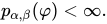
The family of seminorms p_{α, β} defines a locally convex topology on the Schwartz space. When n is equal to 1, the seminorms are, in fact, norms on the Schwartz space. Otherwise, one can define a norm on S(Rⁿ) via

${\displaystyle \|\varphi \|_{k}=\max _{|\alpha |+|\beta |\leq k}\sup _{x\in \mathbf {R} ^{n}}\left|x^{\alpha }D^{\beta }\varphi (x)\right|}$ for k ≥ 1.

The Schwartz space is metrizable and complete. Because the Fourier transform changes differentiation by x^α into multiplication by x^α and vice versa, this symmetry implies that the Fourier transform of a Schwartz function is also a Schwartz function.

The space of tempered distributions is defined as the (continuous) dual of the Schwartz space. In other words, a distribution T is a tempered distribution if and only if

${\displaystyle \lim _{m\to \infty }T(\varphi _{m})=0.}$

is true whenever

${\displaystyle \lim _{m\to \infty }p_{\alpha ,\beta }(\varphi _{m})=0}$

holds for all multi-indicesα, β.

The derivative of a tempered distribution is again a tempered distribution. Tempered distributions generalize the bounded (or slow-growing) locally integrable functions; all distributions with compact support and all square-integrable functions are tempered distributions. More generally, all functions that are products of polynomials with elements of L^p(Rⁿ) for p ≥ 1 are tempered distributions.

To study the Fourier transform, it is best to consider complex-valued test functions and complex-linear distributions. The ordinary continuous Fourier transformF yields then an automorphism of Schwartz function space, and we can define the Fourier transform of the tempered distribution T by (FT)(Ψ) = T(Fψ) for every Schwartz function Ψ. FT is thus again a tempered distribution. The Fourier transform is a continuous, linear, bijective operator from the space of tempered distributions to itself. This operation is compatible with differentiation in the sense that

${\displaystyle F{\dfrac {dT}{dx}}=ixFT}$

and also with convolution: if T is a tempered distribution and Ψ is a slowly increasing infinitely differentiable function on Rⁿ, then ψT is again a tempered distribution and

${\displaystyle F(\psi T)=F\psi *FT\,}$

is the convolution of FT and Fψ. In particular, the Fourier transform of the constant function equal to 1 is the δ distribution.

Under some circumstances, it is possible to define the convolution of a function with a distribution, or even the convolution of two distributions.

Convolution of a test function with a distribution

If f ∈ D(Rⁿ) is a compactly supported smooth test function, then convolution with f,

${\displaystyle {\begin{cases}C_{f}:\mathrm {D} (\mathbf {R} ^{n})\to \mathrm {D} (\mathbf {R} ^{n})\\C_{f}:g\mapsto f*g\end{cases}}}$

defines a linear operator which is continuous with respect to the LF space topology on D(Rⁿ).

Convolution of f with a distribution T ∈ D′(Rⁿ) can be defined by taking the transpose of C_f relative to the duality pairing of D(Rⁿ) with the space D′(Rⁿ) of distributions (Trèves 1967, Chapter 27). If f, g, ${\displaystyle \varphi }$ ∈ D(Rⁿ), then by Fubini's theorem

${\displaystyle \left\langle C_{f}g,\varphi \right\rangle =\int _{\mathbf {R} ^{n}}\varphi (x)\int _{\mathbf {R} ^{n}}f(x-y)g(y)\,dy\,dx={\bigl \langle }g,C_{\widetilde {f}}\varphi {\bigr \rangle }}$

where ${\displaystyle \scriptstyle {{\widetilde {f}}(x)=f(-x)}}$. Extending by continuity, the convolution of f with a distribution T is defined by

${\displaystyle \langle f*T,\varphi \rangle =\left\langle T,{\widetilde {f}}*\varphi \right\rangle }$

for all test functions ${\displaystyle \varphi }$ ∈ D(Rⁿ).

An alternative way to define the convolution of a function f and a distribution T is to use the translation operator τ_x defined on test functions by

${\displaystyle \tau _{x}\varphi (y)=\varphi (y-x)}$

and extended by the transpose to distributions in the obvious way.^[11] The convolution of the compactly supported function f and the distribution T is then the function defined for each x ∈ Rⁿ by

${\displaystyle (f*T)(x)=\left\langle T,\tau _{x}{\widetilde {f}}\right\rangle .}$

It can be shown that the convolution of a smooth, compactly supported function and a distribution is a smooth function. If the distribution T has compact support as well, then f∗T is a compactly supported function, and the Titchmarsh convolution theorem (Hörmander 1983, Theorem 4.3.3) implies that

${\displaystyle \operatorname {ch} (\operatorname {supp} (f*T))=\operatorname {ch} \operatorname {supp} f+\operatorname {ch} \operatorname {supp} T}$

where ch denotes the convex hull and supp denotes the support.

Distribution of compact support

It is also possible to define the convolution of two distributions S and T on Rⁿ, provided one of them has compact support. Informally, in order to define S∗T where T has compact support, the idea is to extend the definition of the convolution ∗ to a linear operation on distributions so that the associativity formula

${\displaystyle S*(T*\varphi )=(S*T)*\varphi }$

continues to hold for all test functions ${\displaystyle \varphi }$.^[12]

It is also possible to provide a more explicit characterization of the convolution of distributions (Trèves 1967, Chapter 27). Suppose that it is T that has compact support. For any test function ${\displaystyle \varphi }$ in D(Rⁿ), consider the function

${\displaystyle \psi (x)=\langle T,\tau _{-x}\varphi \rangle .}$

It can be readily shown that this defines a smooth function of x, which moreover has compact support. The convolution of S and T is defined by

${\displaystyle \langle S*T,\varphi \rangle =\langle S,\psi \rangle .}$

This generalizes the classical notion of convolution of functions and is compatible with differentiation in the following sense:

${\displaystyle \partial ^{\alpha }(S*T)=(\partial ^{\alpha }S)*T=S*(\partial ^{\alpha }T).}$

This definition of convolution remains valid under less restrictive assumptions about S and T.^[13]

The formal definition of distributions exhibits them as a subspace of a very large space, namely the topological dual of D(U) (or S(R^d) for tempered distributions). It is not immediately clear from the definition how exotic a distribution might be. To answer this question, it is instructive to see distributions built up from a smaller space, namely the space of continuous functions. Roughly, any distribution is locally a (multiple) derivative of a continuous function. A precise version of this result, given below, holds for distributions of compact support, tempered distributions, and general distributions. Generally speaking, no proper subset of the space of distributions contains all continuous functions and is closed under differentiation. This says that distributions are not particularly exotic objects; they are only as complicated as necessary.

If f ∈ S′(Rⁿ) is a tempered distribution, then there exists a constant C > 0, and positive integers M and N such that for all Schwartz functions${\displaystyle \varphi }$ ∈ S(Rⁿ)

${\displaystyle \langle f,\varphi \rangle \leq C\sum \nolimits _{|\alpha |\leq N,|\beta |\leq M}\sup _{x\in \mathbf {R} ^{n}}\left|x^{\alpha }D^{\beta }\varphi (x)\right|=C\sum \nolimits _{|\alpha |\leq N,|\beta |\leq M}p_{\alpha ,\beta }(\varphi ).}$

This estimate along with some techniques from functional analysis can be used to show that there is a continuous slowly increasing function F and a multi-index α such that

${\displaystyle f=D^{\alpha }F.\,}$

If f ∈ D′(Rⁿ), then for any compact set K ⊂ Rⁿ, there exists a continuous function F compactly supported in Rⁿ (possibly on a larger set than K itself) and a multi-index α such that f = D^αF on C_c^∞(K). This follows from the previously quoted result on tempered distributions by means of a localization argument.

If f has support at a single point {P}, then f is in fact a finite linear combination of distributional derivatives of the δ function at P. That is, there exists an integer m and complex constants a_α for multi-indices |α| ≤ m such that

${\displaystyle f=\sum \nolimits _{|\alpha |\leq m}a_{\alpha }D^{\alpha }(\tau _{P}\delta )}$

where τ_P is the translation operator.

A version of the above theorem holds locally in the following sense (Rudin 1991). Let T be a distribution on U, then one can find for every multi-index α a continuous function g_α such that

${\displaystyle \displaystyle T=\sum \nolimits _{\alpha }D^{\alpha }g_{\alpha }}$

and that any compact subset K of U intersects the supports of only finitely many g_α; therefore, to evaluate the value of T for a given smooth function f compactly supported in U, we only need finitely many g_α; hence the infinite sum above is well-defined as a distribution. If the distribution T is of finite order, then one can choose g_α in such a way that only finitely many of them are nonzero.

The success of the theory led to investigation of the idea of hyperfunction, in which spaces of holomorphic functions are used as test functions. A refined theory has been developed, in particular Mikio Sato's algebraic analysis, using sheaf theory and several complex variables. This extends the range of symbolic methods that can be made rigorous mathematically, for example Feynman integrals.

It is easy to define the product of a distribution with a smooth function, or more generally the product of two distributions whose singular supports are disjoint. With more effort it is possible to define a well-behaved product of several distributions provided their wave front sets at each point are compatible. A limitation of the theory of distributions (and hyperfunctions) is that there is no associative product of two distributions extending the product of a distribution by a smooth function, as has been proved by Laurent Schwartz in the 1950s. For example, if p.v. 1/x is the distribution obtained by the Cauchy principal value

${\displaystyle \left(\operatorname {p.v.} {\frac {1}{x}}\right)[\varphi ]=\lim _{\varepsilon \to 0^{+}}\int _{|x|\geq \varepsilon }{\frac {\varphi (x)}{x}}\,dx}$

for all ${\displaystyle \varphi }$ ∈ S(R), and δ is the Dirac delta distribution then

${\displaystyle \left(\delta \times x\right)\times \operatorname {p.v.} {\frac {1}{x}}=0}$

but

${\displaystyle \delta \times \left(x\times \operatorname {p.v.} {\frac {1}{x}}\right)=\delta }$

so the product of a distribution by a smooth function (which is always well defined) cannot be extended to an associative product on the space of distributions.

Thus, nonlinear problems cannot be posed in general and thus not solved within distribution theory alone. In the context of quantum field theory, however, solutions can be found. In more than two spacetime dimensions the problem is related to the regularization of divergences. Here Henri Epstein and Vladimir Glaser developed the mathematically rigorous (but extremely technical) causal perturbation theory. This does not solve the problem in other situations. Many other interesting theories are non linear, like for example the Navier–Stokes equations of fluid dynamics.

Several not entirely satisfactory theories of algebras of generalized functions have been developed, among which Colombeau's (simplified) algebra is maybe the most popular in use today.

Inspired by Lyons' rough path theory,^[14]Martin Hairer proposed a consistent way of multiplying distributions with certain structure (regularity structures^[15]), available in many examples from stochastic analysis, notably stochastic partial differential equations. See also Gubinelli–Imkeller–Perkowski (2015) for a related development based on Bony's paraproduct from Fourier analysis.

• Current (mathematics)
• Distribution (number theory)
• Colombeau algebra
• Gelfand triple
• Generalized function
• Homogeneous distribution
• Hyperfunction
• Laplacian of the indicator
• Linear form
• Malgrange–Ehrenpreis theorem
• Pseudodifferential operator
• Riesz representation theorem
• Vague topology
• Weak solution
• Distribution on a linear algebraic group
• Limit of a distribution
• Schwartz-Bruhat function

• Benedetto, JJ (1997), Harmonische Analyse und Anwendungen , CRC PressDie
• Gårding, L. (1997), Einige Analysepunkte und ihre Geschichte , Amerikanische Mathematische GesellschaftDie
• Gel'fand, IM ; Shilov, GE (1966–1968), Verallgemeinerte Funktionen , Bd.  1–5 , Academic PressDie
• Grubb, G. (2009), Distributionen und Operatoren , SpringerDie
• Hörmander, L. (1983), Die Analyse linearer partieller Differentialoperatoren I , Grundl. Mathe. Wissenschaft., vol. 256, Springer, doi : 10.1007/978-3-642-96750-4 , ISBN 3-540-12104-8, MR  0717035Die
• Kolmogorov, A. N .; Fomin, S. V. (1957), Elemente der Funktionentheorie und Funktionalanalysis , Dover BooksDie
• Rudin, W. (1991), Funktionalanalysis (2. Aufl.), McGraw–Hill, ISBN 0-07-054236-8Die
• Schaefer, Helmuth H.; Wolff, MP (1999), Topologische Vektorräume , GTM , Bd. 3, New York: Springer-Verlag , ISBN 9780387987262
• Schwartz, L. (1954), „Sur l'impossibilité de la multiplications des distributions“, CR Acad. Wissenschaft. Paris , 239 : 847–848​Die
• Schwartz, L. (1951), Théorie des distributions , vol.  1–2 , HermannDie
• Sobolev, SL (1936), „Neue Methode zur Lösung des Problems von Cauchy für normale lineare hyperbolische Gleichungen“ , Mat. Sbornik , 1 : 39–72​
• Stein, Elias ; Weiss, Guido (1971), Einführung in die Fourier-Analysis auf euklidischen Räumen , Princeton University Press, ISBN 0-691-08078-XDie
• Strichartz, R. (1994), Ein Leitfaden zur Distributionentheorie und Fouriertransformationen , CRC Press, ISBN 0-8493-8273-4Die
• Trèves, François (1967), Topologische Vektorräume, Distributionen und Kerne , Academic Press, S. 126 ff.Die

• M. J. Lighthill (1959). Einführung in die Fourier-Analyse und verallgemeinerte Funktionen . Cambridge University Press. ISBN 0-521-09128-4(erfordert nur sehr geringe Kenntnisse der Analysis; definiert Distributionen als Grenzwerte von Funktionenfolgen unter Integralen)
• V. S. Vladimirov (2002). Methoden der Theorie verallgemeinerter Funktionen . Taylor & Francis. ISBN 0-415-27356-0
• Vladimirov, VS (2001) [1994], „Verallgemeinerte Funktionen“ , Enzyklopädie der Mathematik , EMS PressDie
• Vladimirov, VS (2001) [1994], „Verallgemeinerte Funktionen, Raum von“ , Enzyklopädie der Mathematik , EMS PressDie
• Vladimirov, VS (2001) [1994], „Verallgemeinerte Funktion, Ableitung von a“ , Encyclopedia of Mathematics , EMS PressDie
• Vladimirov, VS (2001) [1994], „Verallgemeinerte Funktionen, Produkt von“ , Encyclopedia of Mathematics , EMS PressDie
• Oberguggenberger, Michael (2001) [1994], „Verallgemeinerte Funktionenalgebren“ , Encyclopedia of Mathematics , EMS PressDie